Attention mechanism in Deep Learning
In Deep Learning Attention is one component of a network’s architecture, and is in charge of managing and quantifying the interdependence.
- Between the input and output elements (General Attention)
- Within the input elements (Self-Attention)
Let me give you an example of how Attention works in a translation task. Say we have the sentence “How was your day”, which we would like to translate to the French version — “Comment se passe ta journée”.
the Attention component of the network will do for each word in the output sentence is map the important and relevant words from the input sentence and assign higher weights to these words, enhancing the accuracy of the output prediction.

Attention is proposed as a solution to the limitation of the Encoder-Decoder model encoding the input sequence to one fixed length vector from which to decode each output time step. This issue is believed to be more of a problem when decoding long sequences.
there are many different versions of Attention that are applied. We will only cover the more popular adaptations here, which are its usage in sequence-to-sequence models and the more recent Self-Attention
Attention in Sequence-to-Sequence Models
Most articles on the Attention Mechanism will use the example of sequence-to-sequence (seq2seq) models to explain how it works. This is because Attention was originally introduced as a solution to address the main issue surrounding seq2seq models, and to great success. If you are unfamiliar with seq2seq models, also known as the Encoder-Decoder model

A Seq2Seq model is a model that takes a sequence of items (words, letters, time series, etc) and outputs another sequence of items.The most common architecture used to build Seq2Seq models is the Encoder Decoder architecture. This is the one we will use for this post.
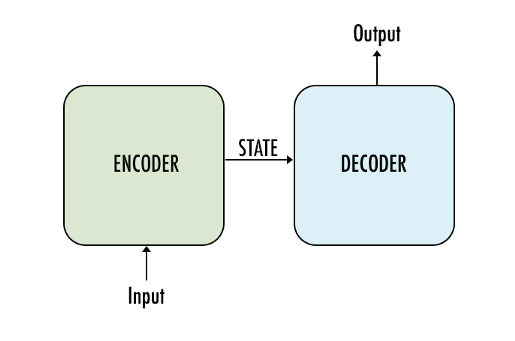
So why does the seq2seq model fails?
So we understood the architecture and flow of the encoder-decoder model since it very useful but it got some limitation. As we saw encoder takes input and converts it into a fixed-size vector and then the decoder makes a prediction and gives output sequence. It works fine for short sequence but it fails when we have a long sequence bcoz it becomes difficult for the encoder to memorize the entire sequence into a fixed-sized vector and to compress all the contextual information from the sequence. As we observed that as the sequence size increases model performance starts getting degrading.
The standard seq2seq model is generally unable to accurately process long input sequences, since only the last hidden state of the encoder RNN is used as the context vector for the decoder
On the other hand, the Attention Mechanism directly addresses this issue as it retains and utilises all the hidden states of the input sequence during the decoding process
Attention model does this by creating a unique mapping between each time step of the decoder output to all the encoder hidden states.
A critical and apparent disadvantage of this fixed-length context vector design is the incapability of the system to remember longer sequences. Often is has forgotten the earlier parts of the sequence once it has processed the entire the sequence. The attention mechanism was born to resolve this problem.
the mechanism allows the model to focus and place more “Attention” on the relevant parts of the input sequence as needed
we must note that there are 2 different major types of Attention:
The differences lie mainly in their architectures and computations.
The aimed to improve the sequence-to-sequence model in machine translation by aligning the decoder with the relevant input sentences and implementing Attention. The entire step-by-step process of applying Attention in Bahdanau’s paper is as follows:
- Producing the Encoder Hidden States — Encoder produces hidden states of each element in the input sequence
- Calculating Alignment Scores between the previous decoder hidden state and each of the encoder’s hidden states are calculated (Note: The last encoder hidden state can be used as the first hidden state in the decoder)
- Softmaxing the Alignment Scores — the alignment scores for each encoder hidden state are combined and represented in a single vector and subsequently softmaxed
- Calculating the Context Vector — the encoder hidden states and their respective alignment scores are multiplied to form the context vector
- Decoding the Output — the context vector is concatenated with the previous decoder output and fed into the Decoder RNN for that time step along with the previous decoder hidden state to produce a new output
- The process (steps 2–5) repeats itself for each time step of the decoder until an token is produced or output is past the specified maximum length
- Producing the Encoder Hidden States(Encoder Layer /RNN -Seq2Seq Layer)
For our first step, we’ll be using an RNN or any of its variants (e.g. LSTM, GRU) to encode the input sequence. After passing the input sequence through the encoder RNN, a hidden state/output will be produced for each input passed in. Instead of using only the hidden state at the final time step, we’ll be carrying forward all the hidden states produced by the encoder to the next step.

Attention Layer performed these next 3 steps

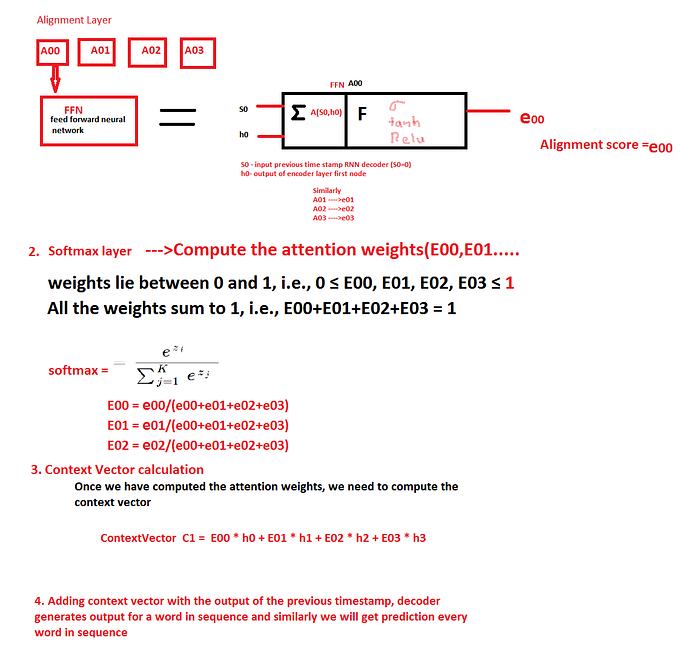
The concept behind Attention(Q,K,V)
Q = Query — ->Decoder hidden state from previous time stamp(S0,S1,S2..)
K = Key — → Hidden state of Encoder(h0,h1,h2…..hk)
V = Value (Normalized weight for calculate the attention weight for C1(context vector)
There are 2 different ways of doing attention mechanisms.these two class depends on how context vector information you need to compress from the input sequence:
- Global Attention
- Local Attention
Let’s dive into these.

Global Attention:
Here, the attention is placed on all the source positions. In other words, all the hidden states of the encoder are considered for deriving the attended context vector. Here we will focus on all the intermediate state and collect all the contextual information so that our decoder model predicts the next word.
Local Attention:
Here, the attention is placed on only a few source positions. Only a few hidden or intermediate states of the encoder are considered for deriving the attended context vector since we only give importance to specific parts of the sequence.
Note : Only one drawback of attention is that it’s time-consuming. To overcome this problem Google introduced “Transformer Model”
Let’s take the same example that used to explain Seq2Seq models
Input (English) Sentence: “Rahul is a good boy”
Target (Marathi) Sentence: “राहुल चांगला मुलगा आहे”
The only change will be that instead of an LSTM layer , here I will use a GRU layer.The reason being that LSTM has two internal states (hidden state and cell state) and GRU has only one internal state (hidden state). This will help simplify the the concept and explanation.

In the traditional Seq2Seq model, we discard all the intermediate states of the encoder and use only its final states (vector) to initialize the decoder. This technique works good for smaller sequences, however as the length of the sequence increases, a single vector becomes a bottleneck and it gets very difficult to summarize long sequences into a single vector. This observation was made empirically as it was noted that the performance of the system decreases drastically as the size of the sequence increases.
The idea behind Attention is not to throw away those intermediate encoder states but to utilize all the states in order to construct the context vectors required by the decoder to generate the output sequence.
Lets represent our Encoder GRU with the below simplified diagram:
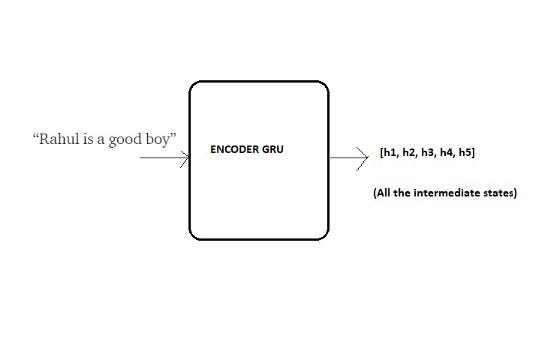
Imagine you are translating “Rahul is a good boy” to “राहुल चांगला मुलगा आहे”. Ask yourself, how do you do it in your mind?
When you predict “राहुल”, its obvious that this name is the result of the word “Rahul” present in the input English sentence regardless of the rest of the sentence. We say that while predicting “राहुल”, we pay more attention to the word “Rahul” in the input sentence.
Similarly while predicting the word “चांगला”, we pay more attention to the word “good” in the input sentence.
Similarly while predicting the word “मुलगा”, we pay more attention to the word “boy” in the input sentence. And so on..
Let’s get technical and dive into the Attention mechanism.
Decoding at time step 1
Continuing the above example, let’s say we now want our decoder to start predicting the first word of the target sequence i.e. “राहुल”
At time step 1, we can break the entire process into five steps as below:
Before we start decoding, we first need to encode the input sequence into a set of internal states (in our case h1, h2, h3, h4 and h5).
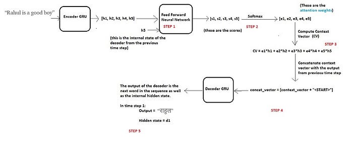
Step 1 — Compute a score each encoder state
Since we are predicting the first word itself, the decoder does not have any current internal state. For this reason, we will consider the last state of the encoder (i.e. h5) as the previous decoder state.
Now using these two components (all the encoder states and the current state of the decoder), we will train a simple feed forward neural network.
we are trying to predict the first word in the target sequence i.e. “राहुल”. As per the idea behind attention, we do not need all the encoder states to predict this word, but we need those encoder states which store information about the word “Rahul” in the input sequence.
As discussed previously these intermediate encoder states store the local information of the input sequence. So it is highly likely that the information of the word “Rahul” will be present in the states, let’s say, h1 and h2.
Thus we want our decoder to pay more attention to the states h1 and h2 while paying less attention to the remaining states of the encoder.
For this reason we train a feed forward neural network which will learn to identify relevant encoder states by generating a high score for the states for which attention is to be paid while low score for the states which are to be ignored.
Let s1, s2, s3, s4 and s5 be the scores generated for the states h1, h2, h3, h4 and h5 correspondingly. Since we assumed that we need to pay more attention to the states h1 and h2 and ignore h3, h4 and h5 in order to predict “राहुल”, we expect the above neural to generate scores such that s1 and s2 are high while s3, s4 and s5 are relatively low.
Step 2 — Compute the attention weights
Once these scores are generated, we apply a softmax on these scores to produce the attention weights e1, e2, e3 ,e4 and e5 as shown above. The advantage of applying softmax is as below:
a) All the weights lie between 0 and 1, i.e., 0 ≤ e1, e2, e3, e4, e5 ≤ 1
b) All the weights sum to 1, i.e., e1+e2+3+e4+e5 = 1
Thus we get a nice probabilistic interpretation of the attention weights.
In our case we would expect values like below: (just for intuition)
e1 = 0.75, e2 = 0.2, e3 = 0.02, e4 = 0.02, e5 = 0.01
This means that while predicting the word “राहुल”, the decoder needs to put more attention on the states h1 and h2 (since values of e1 and e2 are high) while ignoring the states h3, h4 and h5 (since the values of e3, e4 and e5 are very small).
Step 3 — Compute the context vector
Once we have computed the attention weights, we need to compute the context vector (thought vector) which will be used by the decoder in order to predict the next word in the sequence. Calculated as follows:
context_vector = e1 * h1 + e2 * h2 + e3 * h3 + e4 * h4 + e5 * h5
Clearly if the values of e1 and e2 are high and those of e3, e4 and e5 are low then the context vector will contain more information from the states h1 and h2 and relatively less information from the states h3, h4 and h5.
Step 4 — Concatenate context vector with output of previous time step
Finally the decoder uses the below two input vectors to generate the next word in the sequence
a) The context vector
b) The output word generated from the previous time step.
We simply concatenate these two vectors and feed the merged vector to the decoder. Note that for the first time step, since there is no output from the previous time step, we use a special <START> token for this purpose. This concept is already discussed in detail in my previous blog.
Step 5 — Decoder Output
The decoder then generates the next word in the sequence (in this case, it is expected to generate “राहुल”) and along with the output, the decoder will also generate an internal hidden state, and lets call it as “d1”.
Decoding at time step 2
Now in order to generate the next word “चांगला”, the decoder will repeat the same procedure which can be summarized in the below diagram:
The changes are highlighted in green circles

Decoding at time step 3
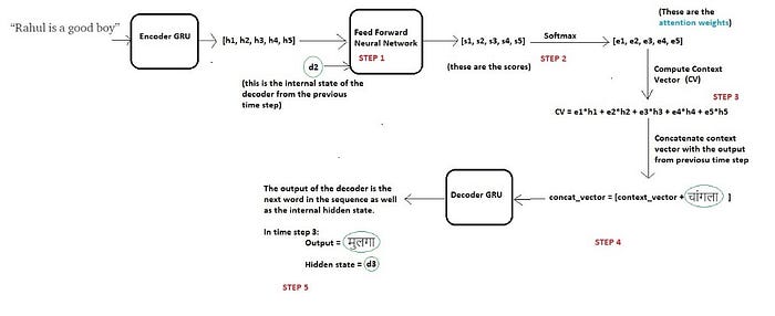
Decoding at time step 4

Decoding at time step 5
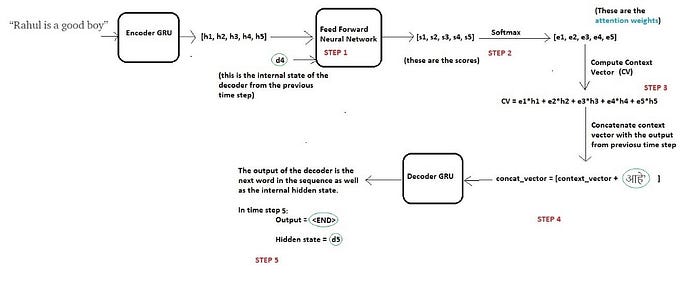
Once the decoder outputs the <END> token, we stop the generation process.
https://lilianweng.github.io/lil-log/2018/06/24/attention-attention.html